 Even old dogs like Excel have some new tricks up their sleeves. The spreadsheet application category was defined by VisiCalc in the late 1970s, and was a driving force behind the success of personal computers; accountants and finance managers and the like could quickly do their own sums instead of waiting for a report from the Data Processing department which fed and watered the big iron. When the PC came out, Lotus 1-2-3 was king of the hill and Microsoft’s Multiplan was an also-ran, until Windows arrived and the new Excel program moved from underdog to top enchilada.
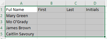
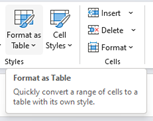
 First off, if you’re going to use Excel to create a table of some sort, start by Formatting as Table. It makes it so much easier to manage the data later – sorting, filtering, formatting are straightforward.
If  you choose that your table has headers, the name of the top row will also be marked with an arrow to filter the list, and also appears in any formulae you might develop.
 Rather than referencing cells in a formula by A2 etc, you could put the cursor onto the field you want to reference, and the name of the column will be used, and when you enter that f
 ormula, it can be easily copied to every row.
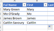
 Excel has other smarts, though – let’s forget about formulae in this case, and just type the First name in column B; dragging the bottom right corner of that cell all the way to the bottom of the table, will fill every cell with “Mary” but a little Auto-Fill Settings prompt will appear at the bottom. Click that and you can change it to Flash Fill.
 Et voila! Excel has figured out the relationship between the text and applied the same
  pattern to all the other rows in the table. Repeat the exercise in this case by filling Green in the Last name and MG in initials. A quicker way of applying auto-fill is to put the cursor in column C and press CTRL-E, then repeat on column D.
If you find yourself working with tables and the columns aren’t wide enough to show the data fully, you can  quickly widen one column by double-clicking on the bar to the side of the column heading; select several colums at the same time and double-click on one of the width adjustors and they’ll all be resized to fit. The same trick works on rows, by double-clicking on the height adjustor on the far left of the row.
If you want to select all the table, put the cursor in the very top left corner of cell A1 and you should see it change shape to a diagonal pointing arrow; click once to select the whole table. Another way would be to put your cursor in the table and press CTRL-A; that selects the entire data portion. Press CTRL-A again if you want to include the header row too.
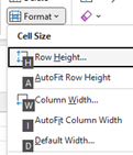
 If you have the table selected, press ALT and release it – you’ll see a load of letters appear over the menus, which jump to specific functions. Press and release H to go to the Home tab, then O to jump to the Format menu, then I for auto-width or A for auto-height.
The final magic Excel trick for today is autocomplete.
If you start typing a text value in a cell, Excel might  look at others in the rows above and offer you an autocomplete option – just
  press tab or downarrow and it will fill in that value for you. Another option is to press ALT and and down arrow ↓ when you first enter or select the cell; it will show a drop-down list of all the previous values, and you can either use mouse or up/down/enter keys to select the one you want. Excellent!
