#31: Easy and Excel-lent Data sources

clip_image002

Most people who have spent time using Microsoft Excel will realize that it probably has more capabilities than they’ll ever understand, much less use. There are so many functions used to collate, display and interpret data that it’s no wonder people turn to using it for all sorts of things.

There have been numerous attempts to make user-friendly data tools for Excel, from web-scraping 3rd party sites to the short-lived Money in Excel for American users which bit the dust before it was barely out of diapers.

More recent releases of Excel include several Linked Data Types which can retrieve and manipulate data from “reputable sources of data, such as Bing”… (which, incidentally, had its 15th birthday recently). Companies with suitable data governance can expose internal info for analysis, or regular end users can get started with share prices, currency conversions and geographical data.

clip_image004

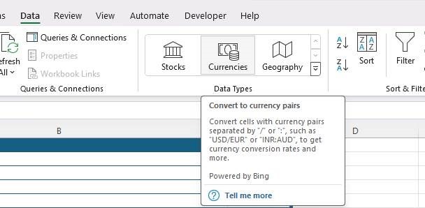
In the Data tab in the current versions of Excel on multiple platforms, you’ll see 3 or 4 types of data that can quickly be inserted – they will perform a lookup on external information and return a data set in the background which can be displayed and otherwise interacted with using formulae, lookups and other standard data tools in Excel.
clip_image006

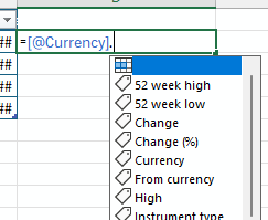
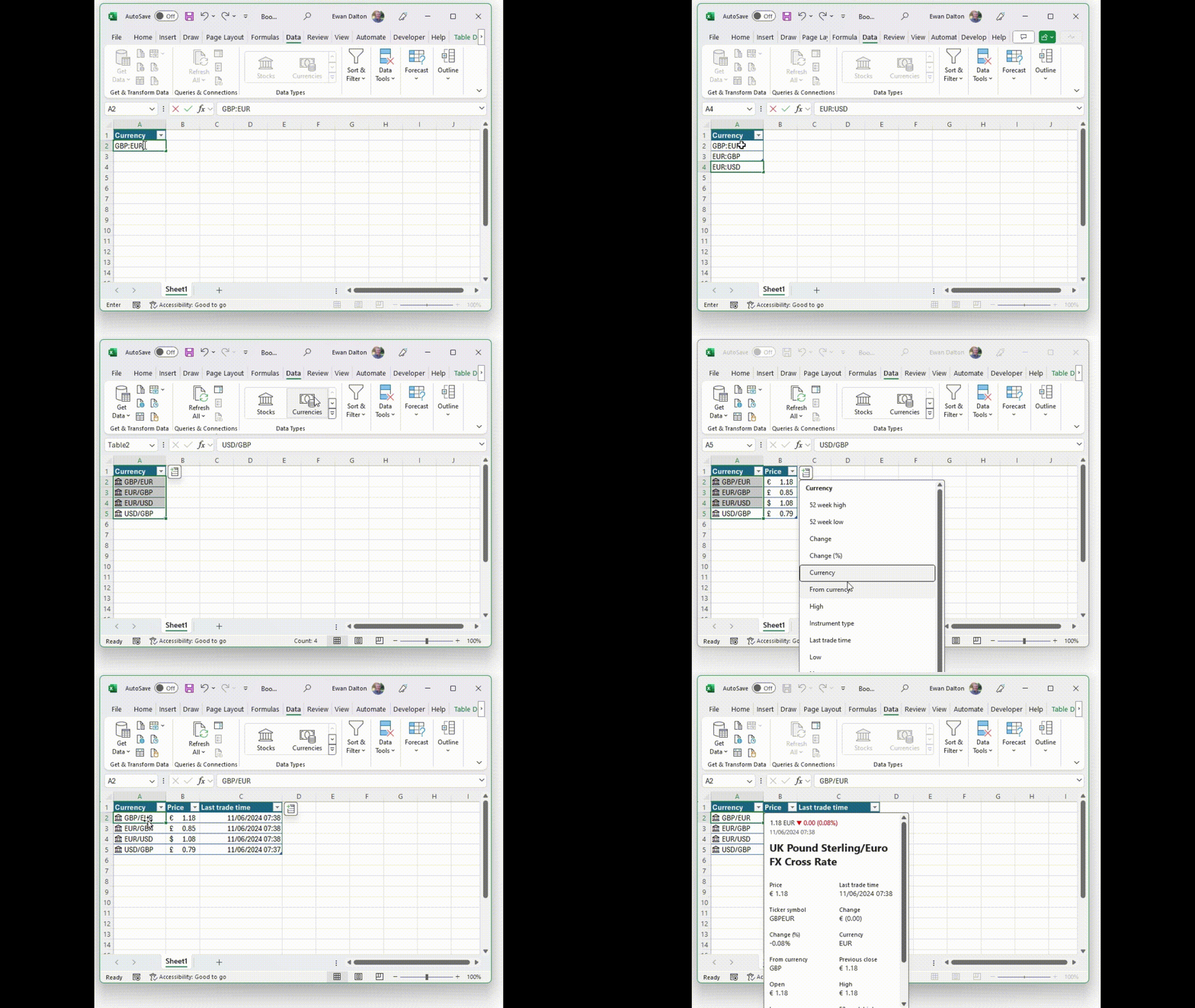
Getting real-time data is pretty straightforward – create a blank table with a single column in which you’ll enter your key data items that you want to expand on – for currency conversions, it would be a pair of currency symbols (USD:EUR or GBP/USD etc) that you then select and mark as Currency from the data tab. That then lets you easily add other columns for specific lookup data, and that can be referenced itself through other formulae too.

clip_image007

Stock lookups work similarly, by entering the ticker symbol in one column and potentially going through a matching exercise to find the right one. Handy, if you have a workbook for calculating when you can stick it to the man and retire to a patch in the Tuscany hills: you can automatically look up the stock values and convert their currencies too, if required.

clip_image009

There’s some location stuff as well, invoked by entering city or area names; it’s more text-based reference info which is returned, though it might be possible to feed some of the data into a Map Chart for further visualization.

671 – Excel-lent

imageEven old dogs like Excel have some new tricks up their sleeves. The spreadsheet application category was defined by VisiCalc in the late 1970s, and was a driving force behind the success of personal computers; accountants and finance managers and the like could quickly do their own sums instead of waiting for a report from the Data Processing department which fed and watered the big iron. When the PC came out, Lotus 1-2-3 was king of the hill and Microsoft’s Multiplan was an also-ran, until Windows arrived and the new Excel program moved from underdog to top enchilada.

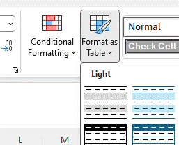
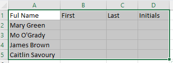
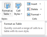
clip_image001First off, if you’re going to use Excel to create a table of some sort, start by Formatting as Table. It makes it so much easier to manage the data later – sorting, filtering, formatting are straightforward.

If clip_image003you choose that your table has headers, the name of the top row will also be marked with an arrow to filter the list, and also appears in any formulae you might develop.

clip_image004Rather than referencing cells in a formula by A2 etc, you could put the cursor onto the field you want to reference, and the name of the column will be used, and when you enter that fclip_image006ormula, it can be easily copied to every row.

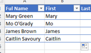
clip_image007Excel has other smarts, though – let’s forget about formulae in this case, and just type the First name in column B; dragging the bottom right corner of that cell all the way to the bottom of the table, will fill every cell with “Mary” but a little Auto-Fill Settings prompt will appear at the bottom. Click that and you can change it to Flash Fill.

clip_image009Et voila! Excel has figured out the relationship between the text and applied the same clip_image011pattern to all the other rows in the table. Repeat the exercise in this case by filling Green in the Last name and MG in initials. A quicker way of applying auto-fill is to put the cursor in column C and press CTRL-E, then repeat on column D.

If you find yourself working with tables and the columns aren’t wide enough to show the data fully, you can clip_image013quickly widen one column by double-clicking on the bar to the side of the column heading; select several colums at the same time and double-click on one of the width adjustors and they’ll all be resized to fit. The same trick works on rows, by double-clicking on the height adjustor on the far left of the row.

If you want to select all the table, put the cursor in the very top left corner of cell A1 and you should see it change shape to a diagonal pointing arrow; click once to select the whole table. Another way would be to put your cursor in the table and press CTRL-A; that selects the entire data portion. Press CTRL-A again if you want to include the header row too.

clip_image015

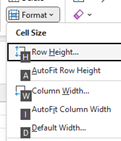
clip_image017If you have the table selected, press ALT and release it – you’ll see a load of letters appear over the menus, which jump to specific functions. Press and release H to go to the Home tab, then O to jump to the Format menu, then I for auto-width or A for auto-height.

The final magic Excel trick for today is autocomplete.

If you start typing a text value in a cell, Excel might clip_image019look at others in the rows above and offer you an autocomplete option – just clip_image021press tab or downarrow and it will fill in that value for you. Another option is to press ALT and and down arrow when you first enter or select the cell; it will show a drop-down list of all the previous values, and you can either use mouse or up/down/enter keys to select the one you want. Excellent!

#639 – Macros, Ghosts and GALs

VB and MacrosSince the early days, Microsoft always kept an eye on what its competitors were doing. It was once de rigeur to produce “battlecards” which would show feature-by-feature how one product is better than its competitor, thus assuring the customer they should buy this one. Thankfully, times have mostly moved on to just building as good a product as possible and then let customers and the markets decide – sometimes, they get improved and honed over time to be the best out there, and sometimes they get dispatched to the boneyard as times move on.

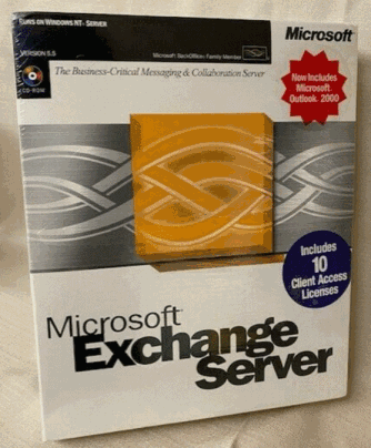
Exchange Server boxIn the late 1990s, Office and Exchange (and later, SharePoint) Server were seen as Microsoft’s entrants into the burgeoning “Groupware” market, which became subsumed into “Knowledge Management” c2000. Key competitors to Exchange & Outlook were Lotus Notes and Novell GroupWise, both of which came from being collab tools and gained email functions. Notes was arguably much more mature and feature rich even if the UI was sometimes clunky, GroupWise was much leaner but found a niche in several industries. Amazingly, GroupWise is still a thing and Notes evolved first into IBM Notes/Domino and was eventually sold off to now be HCL Notes and HCL Domino.

One of the early moves Microsoft made to elevate Office apps to more than just writing documents, was to try to make the docs more capable through adding Macros, and later, Visual Basic for Applications. This allowed a moderately skilful user to dabble in programming to make smarter applications centered around documents; what seemed like a good idea at the time unwittingly unleashed a wave of malware, where bad actors wrote macros to do undesirable things. Following the “Melissa” worm in 1999, Office stopped Macros running without asking the user for permission. Using Macros for anything more than tinkering never really took off.

Blocked Macro warning

Macros disabled entirely

Microsoft announced in February 2022 that all Office Macros in content received online would be disabled completely; this was temporarily rolled back in some test builds for some changes to be made in how it works, but for many, the warning will still be there if you open a Macro-enabled file that you’ve downloaded or been sent.

Unblocking MacroThere are still some very useful Office macros out there, and if you do need to run one that you know is from a trustworthy source, there is a workaround – save the file to your PC locally, then right-click on it to look at the file’s properties, tick the “Unblock” option and apply that. You’ll now be able to choose to run the macro unencumbered.

One such handy macro was discussed back in December 2021 in ToW 611, and is used to find Ghost meetings – ie ones you have arranged but everyone has declined (or at least not accepted). The macro spins through all future meetings in your calendar and lists the ones you’ve organised but where you’re likely to be the only attendee who shows up. Particularly useful at this time of year if lots of people are about to take time off over the summer, and may have declined a few recurring meetings but you – as organiser – still have them in your calendar.

Ghost Meetings

For the latest version of the macro, download the ZIP file to your machine and expand it (or just copy the XLSM file that’s within and put it somewhere else), do the property Unblock thing as above, open in Excel, click the button to allow content, then the Scan Calendar button and you’re all set. You still need to go into Outlook and look at the appropriate date then decide if you want to cancel those meetings or not.

Another more powerful macro – though a little more esoteric – is one which does bulk resolution against the Global Address List, so if you give it a list of display names and/or alias names, it will show the full name, title, department, office, email, and alias name of that person. Handy if you want to get the full details of everyone who is going to attend a meeting, but if you just have a longish list of names then you could just paste them in and see how it goes. This was covered back in ToW 575. One usage scenario recently was to estimate the number of people who were attending a group meeting, but were based at other offices and would therefore need accommodation.

Here’s an example output of over 500 names who were invited to a large meeting; by just providing their display names in column A, it took the sheet about 30 seconds to complete, with 10 identified as distribution lists and 50 unknowns who couldn’t be resolved, either due to no longer being in the GAL or because there were more than one possible name listed.

GAL resolving

If you can manually find the unknown person/people in the GAL, then get their alias name and paste that into column 1 instead of the ambiguous display name, then try to run it again.

623 – What’s .new pussycat?

clip_image002Many products evolve due to exposure to their competitors – adopting and refining the best features, and sometimes that evolution even starts to overtake the original. Many traditional desktop applications moved to online variants or were supplanted by newer concepts, such as shifting to mobile apps. Experiences that were clunky – like banking – moved to sometimes lower-functionality but more convenient apps, just as consumers adopted mobile payments and contactless cards.

Having blazed a trail with email in Hotmail and later Outlook Web Access, in 2010 Microsoft launched the first version of the Office web applications, meaning you could run lightweight Word, Excel and PowerPoint in your browser, as a companion or even as an alternative to the full-fat desktop versions.

A few years earlier, Google Docs released as an online word processor (and later, other types of productivity apps, rebranding as G Suite and now Google Workspace). There are pros and cons of the browser-only experience; you tend to sacrifice some functionality compared to the desktop applications in favour of ubiquitous availability, though web clients can be updated more easily and sometimes new features appear there first – as ToW #605 covered, with snoozing email.

Check out What’s new in Excel for the web or look for the summary covering Visio, Forms, Words and more, here.

clip_image004Not sure about living in a browser? Modern-living afficionados can get by, using only web apps like Outlook, OneNote, To-Do and more.

If you like being browser based rather than desktop boundclip_image006, you could start a new document from the address bar by simply entering word.new, excel.new or powerpoint.new. Others include docx.new, ppt.new, teams.new, sway.new

clip_image008You could add such links to your browser favourites; therefore, a new doc is but a single click away.  There are many more .new shortcuts – Google’s in-house domain registry launched the service a few years ago, so not unsurprisingly, Mountain View hoovered up a lot of the relevant ones if you’re of a Googly persuasion. See docs.new, sheets.new or slides.new, mail.new

597 – Pivot table filtering

clip_image002Pivot Tables are a somewhat esoteric spreadsheet feature which everyday Excel users probably shy away from, but for the enlightened can help to turn potentially large tables of raw data into summarised views that can be easily rearranged.

Excel makes it easy to take a static table with rows of data arranged into columns that correspond to measures or fields – like sales of a product, or assignments of a relationship such as an export from a CRM system – and then represent the inherent hierarchy in a super-powerful fashion.

If you haven’t really used Pivot Tables, the simplest way to get your head around what they can do is to try messing around with some real data, or use some relatively simple sample data to unearth the power within. Free sample data at Contextures is a good place to start – in fact, here’s one sample that has been turned into a Pivot table to get started with (just download it somewhere, open the Zip file and then open the example XLSX file within).

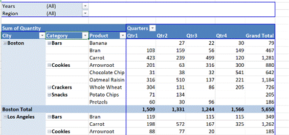
clip_image004The sample data is sales of foods over a period of time; look at the FoodSales tab to see the raw data. The pivot table quickly lets you summarise by region, or category, or whatever fields are defined.

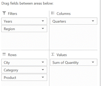
By showing the PivotTable field list (right-click on the table and you’ll see either show or hide field list at the bottom of the menu), you can easily drag things around to change the grouping order.

clip_image006It’s easier to just try it out than to try and explain, though there are plenty of tutorials around – from overviews to walkthrough videos or all kinds of more advanced stuff. And if you end up making a mess of the table, there’s also CTRL+Z to undo…

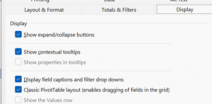
clip_image008If you’re dealing with lots of fields that would go in the Rows section then you might find it easier to use the Classic layout by right-clicking on the table and choosing Pivot Table options, though you might want to remove the auto-totalling for most of the fields (right-click on a field and choose Subtotal…) otherwise the display gets a bit unwieldy.

clip_image010When handling very large volumes of data, filtering using the drop-downs to the right side of field names is a great way of showing only the specifics you’re interested in, though sometimes it’s easy to forget there’s a filter in force and think that the data you’re working with is not showing the full picture. To reset all the filters back to the start, just go to the Data tab and Clear the filters from there.

clip_image012If you want to filter on a specific value – eg. Let’s say you have a list of customer account names and you want to show only the customers associated to a single account manager (regardless of geography, industry etc), you could click the filter on the account manager field and find the person’s name within.

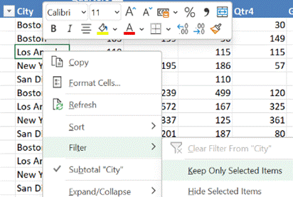
In our foodstuff example, we could have a different layout of fields and want to filter on City – but a quicker way to doing so is to just right-click on the name you want to focus on, and choose Filter > Keep Only Selected Items and it will quickly set the filter to just that name.

593 – It’s a Date

clip_image002Following last week’s missive on Notepad, including the obscure tip on how to create a log file, the topic of inserting and handling dates in other applications is worth a (re-)visit. Each individual app may choose to offer different methods and formats, but for common Office applications there are a handful of memorable tricks and shortcuts.

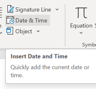
clip_image004In Word, there are plenty of ways to insert and manage dates – perhaps the most useful way to remind the reader when the document was last updated (manually showing when a document was last reviewed or published). On the Insert tab, you’ll find Date & Time on the right-hand side, letting you add appropriate info in the format of your choice. You can also tick a box to update the field automatically, though that simply means every time the document is opened, it will show today’s date… which feels a bit pointless.

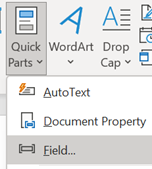
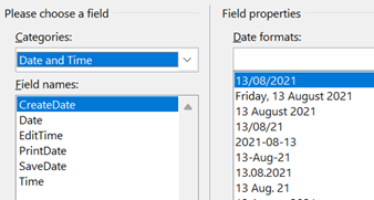
clip_image006More useful could be to tell the reader when the document was created or last saved, by referencing the actual properties of the document clip_image008(though be careful; auto-save might mean someone opened an old document, realised it was irrelevant, but had inadvertently saved it back).

On the Insert tab / Quick Parts, look under Field, then pick the doc property and format you’d like to show.

It is worth pointing out that showing a date as 10/1/21 (or similar) is ambiguous given that a few hundred million people will expect it be month-day-year while many of the remaining 7 billion will assume the day comes first, with a couple of billion presuming the format should normally start with the year, such as yyyy-mm-dd (which is arguably the most sensible of all; and it sorts properly, too).

A more daily usable short format like dd-mmm-yy (ie 13-Aug-21) should perhaps be the norm, especially when the date is appearing as text in a document. Pressing SHIFT+ALT+D in Word will insert the current Date as a field (so you can edit the format to remove ambiguity) and SHIFT+ALT+T inserts the current time too. In PowerPoint, both of these combos bring up the “Date & Time” dialogue to add the chosen content and format as plain text.

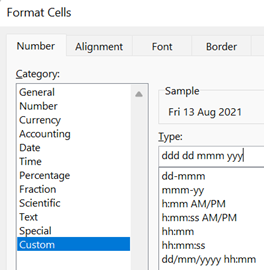
clip_image010When formatting dates, incidentally, the convention is that two letters refer to the short number (eg dd = 13), whereas 3 d’s or m’s will use the short form of spelling the day or month, with 4 meaning the whole thing (ie Friday, August). Try formatting a cell in Excel as Custom, and you can preview what the format would be, by typing in a variety of letters.

While in Excel, it’s worth learning the short cut key to insert the date and time – CTRL+; and SHIFT+CTRL+; respectively (no doubt there’s a reason why Excel has a different shortcut to other Office apps – some legacy of Lotus 1-2-3 perhaps?).

OneNote fans will want to remember that SHIFT+ALT+D / T combo as it inserts the date/time into the notebook; really handy when taking notes of a phone call or similar. SHIFT+ALT+F puts both day and time, something that Word doesn’t offer. In both Desktop OneNote and users of the Windows Store version, it’s just plain text that gets added, so you’re on your own when it comes to formatting.

clip_image012

OneNote pages will typically have a date & time showing under their title – on the Desktop version, it’s possible to change that so as to mark a page as having been recently updated. No such luck on the lame duck Store version.

At least when stalwarts insist on writing – or worse, saying – a short-form date as something like “ten one”, there’s more than half of each month where one number in the date could only mean “day” – starting with the thirteenth (as in, 8/13 can never by the 8th of a month, but 8/12 could be a few days before Christmas to Europeans, or the date when tweedy Americans start looking for grouse in the Yorkshire moors and Scottish Highlands).

591 – An Excel Smörgåsbord

clip_image002Think of this week’s tip as not one single dish, but rather a series of related snacks; a groaning table of cold hors d’oeuvres or sizzling spicy tapas, with one common theme – they’re all about Excel.

May the F4 be with you

One of the neatest features in Office yet largely hidden; the F4 key repeats the last command without needing to faff about selecting the option from the menu. So what, you might say? Well, what if you’re formatting cells and want to repeat the same format over and over again – you could change one, then use the Format Painter option to apply that to select other cells, or possibly just apply the format you want, then select each additional cell in turn and press F4.

One slight downside is that it only repeats the very last action, so changing a number format and then making it bold wouldn’t be easily repeatable since those are two actions. Still, there are so many uses for this “Magic Key no one knows about”.

CTRL+y does the same thing in case you’ve got one of those annoying keyboards where the function keys do other things, you never know without looking if you’ll be pressing F4 or changing the system volume.

Layouts and Tabs

Now, Windows has lots of tricks for arranging application windows side by side, especially if you have multiple monitors; there’s a particularly shiny new way of doing it in Windows 11 with Snap Layouts. In the context of Excel, that’s OK if you’re using two spreadsheets side by side and you might want to reference or copy data between them, but Excel has its own window-handling functions that could be more useful.

clip_image004The key scenario here is that you can open the same document in more than one window (by clicking New Window, on the View tab) and then show different parts of it side/side – separate tabs, perhaps, or different areas on the same sheet.

The Synchronous scrolling feature means clip_image006you can also keep the cursor at the same point in both sheets, making it easier to compare. If you have functions on one tab that depends on data from another, you could change the data in one window and see its impact in real time in the other.

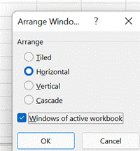
Click on the Arrange All menu option to automatically distribute the open Excel windows, optionally confining the process to just the windows from the active workbook.

Transpose data with paste

It’s a fairly common exercise to take a load of data that’s in one format and want to represent it differently; there is a useful Transpose feature that takes data from columns and paste it back as a row, or vice versa. One useful scenario could be when you want to take the names of everyone who got an email or meeting request and put them in a tabular format.

clip_image008Start by copying and pasting the names/addresses from Outlook’s To: field into a new cell: you’ll see that is’ one long string of text that needs to be broken down, but in this case, each address is delimited with a semicolon (“;”).

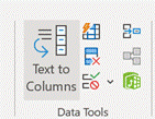
clip_image010Having selected the cell, go to the Data tab in Excel and choose Text to Columns then choose clip_image012Delimited and select the semicolon. Once the wizard is complete, you’ll end up with each address in its own column. Now select the multiple cells and copy to clipboard.

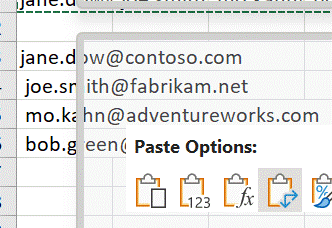
clip_image014Next, put the cursor on a lower row or maybe a new sheet altogether; right-click on the destination cell and under Paste Options, look for the Transpose icon (with the two arrows); hovering over the different icons in this menu will preview what you’re going to do. Click on the icon to commit.

Now you have a list of addresses on their own row, and without the “;”s, but they do have a leading space ahead of all but the first one. It might be quick to correct each line in turn, and there’s always the TRIM function which could be used to tidy stuff up through formulae.

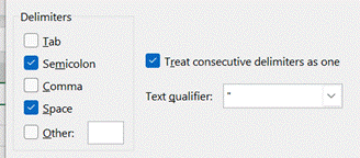
clip_image016Alternatively, go back to the start of the process, select both Semicolon and space, and choose to combine the two, so the text in the columns is neater.

When you’re happy, remove the original line that had the text in columns, leaving just the separate email addresses on their own rows.

Now, snacks just make you hungry, don’t they?

587 – New Line please

clip_image002Lots of terms in computing have their roots in an earlier time, where the association has long since disappeared. The mouse was so called because of its “tail” connecting it to the machine; when was the last time you used a wired mouse? Then there’s the apocryphal story of a young person, on first encountering a 3.5” floppy disk (er, not so floppy any more) thinking that someone had 3D printed the save icon.

As well as the QWERTY keyboard layout, a few things were carried over to the modern computer from the typewriter – the backspace and tab keys and the carriage return key. Purely mechanical typewriters had an end-of-clip_image004line lever, which caused the paper to feed one line and the whole mechanism of the roller to shoot back to start a new line. Electric typewriters had the innovation of not requiring the dings and the manual whirrs, by pressing the RETURN key to automate the carriage – the symbol still displayed on most computer keyboards today is indicative of the physical action.

Early computer systems aped the same approach of the line feed (ie the paper being shuffled up one line) and the carriage return (going back to the left side), as being separate activities and they were given specific control codes – so CR, LF and CR+LF are still things. For some time, consternation still applied as Windows considered that CR + LF needed to be noted to really start a new line, whereas the Unix fraternity simply thought that LF was all you needed. It is possible to hack the registry so Notepad acts Unixsy should you need it to.

In most applications, if you want to start a new line, you’d just press Return or Enter (in effect, the same thing, though not always the case). Pedants would say that ENTER doesn’t mean you necessarily need a new line, you’re just committing some data you’ve typed, redolent of the old terminal where you might be submitting a form rather than typing in free text.

Applications perform sometimes completely different actions when you press a modifier key like CTRL or ALT, and ENTER. In Word, CTRL+ENTER starts a new page, ALT+ENTER repeats the last typing action. In Outlook, CTRL+ENTER sends the current email and ALT+ENTER – like the same keystroke normally does when looking at a file in Windows Explorer – shows the properties of the current message.

In Excel, CTRL+ENTER has some other meanings, notably it completes the entry of data into a cell, without moving the selection to the next cell along or to the line below (depending on config). SHIFT+CTRL+ENTER can be used to create a powerful but quite complex array formula. ALT+ENTER also has a useful trick for formatting text in-cell, alongside some tips to control cell text formatting.

clip_image006Firstly, wrap text where it makes sense – so clip_image008to stop it spilling into the next column and getting over-written by whatever text is or may be added in there.

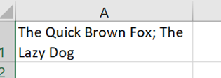
clip_image010Sometimes, however, the layout doesn’t quite sit right unless you resize the column, and that might not be ideal. If typing in new text into a cell, you can force a new-line within the box by pressing ALT+ENTER. For existing text in a cell, one solution to put a new line in is to double-click in the cell, which will insert a flashing text cursor and you edit text directly in the cell rather than the formula bar text box at the top of the sheet. Move the cursor using the arrow keys clip_image012and/or by clicking the mouse elsewhere in the text; press ALT+ENTER  to force a new line in the box.
Much neater.

Another way of editing text in an existing cell; select it and the text will be displayed in the formula bar, but only the first line, unless you have the formula bar expanded out, by clicking the down-arrow on the right.

clip_image014If you show it as a multi-line view, it may be easier to click within that box to edit the text, move the cursor around and hit the ALT+ENTER shortcut to force a new line.

548 – A-List listings

clip_image002Updates flow to Microsoft 365 on a regular basis – there’s a published list of all the minor and major changes that are launched and on their way. As well as improving the current user experience and adding new features, occasionally whole new offerings are added – such as Microsoft Lists, which first made an appearance in July.

Lists gives an easy way of creating, sharing and managing lists of custom clip_image004information within a team – tracking issues, recording assets, anything in fact, that might have used a shared spreadsheet to do it in a low-tech way. Lists was announced to provide a modern-looking, consistent way of managing lists through a variety of front-ends – including mobile apps, to come later this year.

You should be able to see Lists from the menu on Office 365 web apps – start clip_image006at www.office.com and sign in with a business Office/Microsoft 365 login and the new icon will give you access to Lists – get started here.

Just like sharing forms or doing task management, there are often numerous ways to do the same thing – and in days of yore, that would have meant several competing and incompatible technologies, encouraged to fight it out with each other to try to ensure that the best one wins. Nowadays, with a more collegiate mindset, consistent ways of doing things show up in different user experiences – like To-Do and Outlook, StickyNotes and more. Expect deeper integration across other apps in due course

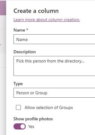
The new Lists experience is essentially just a great UI built on top of a mature back-end; SharePoint Lists, which have evolved over the last 10+ years, allowing the definition of custom columns and rules to validate data entry.

One new frontier is to integrate the new Lists UI into Teams; if you have ability to administer a Team, clip_image008you will see an “add a tab” function alongside the Posts / Files etc tabs that are typically presented.

clip_image010Adding a List tab will then walk you through a process to either choose an existing List (by entering the URL of the SharePoint site that hosts it) or by creating one by importing a spreadsheet, starting from a number of templates or by defining it from scratch

Have a play with Lists and think about how your team could use them in place of spreadsheets.

Microsofties: There’s an internal story about how Lists came about, and looking forward to where it’s likely to go in the future.

Check out Paul Thurrott’s excellent introduction to Lists. And there’s even a Lists Look Book.

542 –Excel Special Paste

clip_image002
Anyone who spends an amount of time preparing spreadsheets in Excel, will be familiar with the frustrations that can come from cut, copy & paste. You need to know what the source of a cell is before you know how it will behave if you copy and paste it somewhere else, even to another sheet.

As an example, if you took the small table below and wanted to copy and paste the calculated values on row 4, you’d need to deal with the fact that the formula will change – offsetting the D and the 2 reference to wherever you paste it (eg if you pasted the copy into E4, the formula would be =E2-E3) – normally, a powerful and useful function, but a potential nuisance.

clip_image004You could decide to paste just the value itself (which means that if the values in D2 and D3 changed, cell D4 would be recalculated but your copy would not), or you could copy the cell, then copy original cell’s formula and paste that into the formula of the destination cell.

clip_image006There are lots of “Paste Special” options, which will vary depending on what kind of data is in the clipboard. Right-click in a destination cell and the Paste Options menu will surface the commonly used variants, or click the arrow by Paste clip_image008Special to see all the others. Move the mouse over that pop-up menu and the rest will fade away.

An older UI for selecting the options is available if you click on the Paste Special… command at the bottom of the pop-out, or by pressing CTRL+ALT+V to pop out the Special dialog.

clip_image010Transposing

One of the more particularly useful features of Paste Special in Excel is the Transpose option – if you select and Copy a row of data then Paste / Transpose it, the data is rearranged as a column (and vice versa). Great news in many cases, but if you want to paste cells and keep the original formulae (without resorting to using absolute references formula references using $ in the formula itself, eg setting =$D$2-$D$3), there are no default options to transpose the orientation of the cells but not change the  formulae.

clip_image012

One trick if you ever find yourself in this position, is to bulk change the formulas so they won’t get modified when you paste the cells; do a Find & Replace to change = to something like #=.

After pasting and transposing, reverse the process to restore the formulaclip_image014.

clip_image016NB: this can be a little hit and miss depending on how you’re using cell names or references – you may find that it’s more reliable if the reference is made to a cell on a different worksheet.

It’s an edge case but could save you lots of time if you need to do it.

For most of us, getting to grips with shortcut keys in Excel would make things more productive – as well as numerous combos of CTRL-something, there are simple keys (like pressing F4, which repeats the very last command … so if you’ve just coloured a cell yellow, move the cursor to another cell and hit F4 to make that one yellow too… if you’re doing very repetitive things, this can save so much time).

There are also more complex sequences; press the ALT key in Excel (and other Office apps, too) to see the key combos that clip_image018invoke each command group on menus or the Ribbon – if you can’t remember the shortcut, just press ALT then the key for the menu you want, then the key on the menu that equates to the command you’re looking for.

clip_image020

A little bit of legacy/history – press ALT-E then S to jump to the Paste Special menu – why E? Even though it’s long gone, really old versions of Excel had an Edit menu, and the commands on any menu – in any application – that have an underscore under a letter (like Paste Special) are highlighting the key you can press to jump to that command.

So ALT E / S used to be the combo to get Paste Special circa Excel 2003, and it still exists today.